Nine different RANS turbulence models are compared in STAR CCM+ 2020, using the mixing plane data from the NACA database [1]. Seven of these models are compared on turbulent kinetic energy, while all nine models are compared on velocity. The models that are used are summarized in the list below, models with a * are compared both on velocity and turbulent kinetic energy.

Geometry

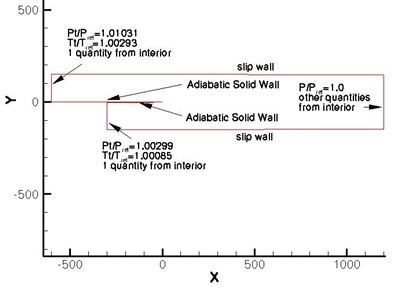
The (2D) geometry consists of two inlets with two velocities (the top inlet has a velocity of 41.54 m/s while the lower inlet has a velocity of 22.4 m/s). The upper inlet channel is longer than the lower inlet channel. A plane keeps the upper and lower inlet channels separated up to x = 0. The plate has a thickness of 3mm and is tapered to a thickness of 0.3mm in the last 50mm. This geometry is the same as the geometry used in the reference, see the figure below [1].

The reference temperature, T_ref, is 293K, the speed of sound, a_ref, is 343 m/s and the reference pressure, P_ref, is 101325 Pa. A low freestream turbulence level of 0.3% is used.

Mesh

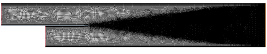
Because Femto usually uses unstructured meshes when working with CFD problems an unstructured mesh is used for this problem. A maximum cellsize  of 10mm is used, while the wake of the splitter plate is refined using meshcells with a size of 1.25mm.

Prism layers are used to get the y+ value on the walls to <1.

Results

In Figure 1 the velocity profile at 200mm from the splitter plate is shown. The y value is normalized using the vorticity thickness δ_ω, which is calculated using the equation below.

δ_ω=(U_2-U_1)/(δU/δy)

The y values are corrected using the equation y_corrected=y-0.00688x. Finally the velocity is normalized as well using the equation below.

U_norm=(U-U_1)/ΔU

The results of the CFD calculations are compared to experimental data [2].

All turbulence models show a reasonably good fit with the experimental velocity at x = 200mm. However, the realistic k-ε  model best predicts the change in velocity between -0.2>y/δ_ω >-0.6. The other models which also have a reasonable comparison with the experimental results are the High Re SA model, the SST k-ω model, the standard k-ε model and the realistic k-ε two layer model.. The other models do not predict any sudden change in velocity.

None of the nine turbulence models accurately predicts the velocity profile at x = 650 mm (Figure 2). The models which come closest to the experimental data are the Standard k-ω model and the Quadratic Reynolds stress model.

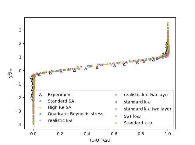
Figure 1: Velocity profile at x = 200mm

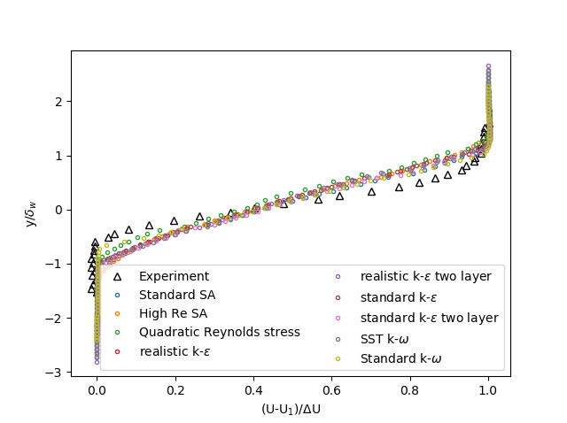
Figure 2: Velocity profile at x = 650mm

The turbulent kinetic energy is normalized using the square root of the difference in velocity. Since both Spalart Allmaras (SA) models did not give any turbulent kinetic energy as output these models are not compared for the turbulent kinetic energy.
In Figure 3 the turbulent kinetic energy at x = 200mm of the seven turbulence models is compared with the experimental data. In this figure it is visible that none of the models accurately predict the point where the turbulent kinetic energy starts to increase. The Standard k-ω, SST k-ω, and the realistic k-ε two layer models all come closest in the prediction of the maximum turbulent kinetic energy. The maximum kinetic energy predicted by the Quadratic Reynolds stress model is similar to the other three models but the position in y is off. The other three models predict a maximum turbulent kinetic energy which is much higher than the experiments.

In Figure 4 the turbulent kinetic energy at x = 650mm is shown. In this case the turbulent kinetic energy behaviour is best predicted by the standard k-ε  and the realistic k-ε models, both in width and in height. The other models predict a maximum turbulent kinetic energy value which is too low and/or a too early y-value where the turbulent kinetic energy starts to increase.

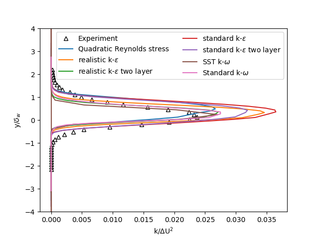
Figure 3: Turbulent kinetic energy at x = 200mm

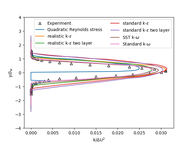
Figure 4: Turbulent kinetic energy at x = 650mm

References

1. https://turbmodels.larc.nasa.gov/delvilleshear_val.html
2. http://cfd.mace.manchester.ac.uk/cgi-bin/cfddb/prpage.cgi?34&EXP&database/cases/case34/Case_data&database/cases/case34

Want to know more?

We have a team of professionals with extensive knowledge that are happy to help. For any questions, use the form below to get in contact.

Contact us