Example
To demonstrate the differences between the two methods we have created a test-case. The test-case consist of the hydrograaf (or pakjesboot). In this simulation 2 exhaust channels are present (as visualized in red in Figure 1), as well as 4 cabin inlets. It is undesired to get exhaust gas within the cabin, therefore we are interested in how much of our exhaust gas reaches the inlets of the cabin.
 Figure 1: cabin inlets and exhaust outlets on the hydrograaf
Each cabin inlet has an air intake of 2kg/s, while each of the two outlets have a velocity of 1.28m/s and an exhaust temperature of 300C. An atmospheric boundary layer makes sure that the velocity of the wind around the ship is modelled correctly, where the wind speed is taken as 3.5 m/s, with an angle of 30° (note that this is a combination of the velocity of the ship and the wind velocity coming at an angle). This angle allows us to determine the exhaust gases that will come into the cabin through the two starboard inlets (shown in light and dark purple in Figure 2).
Even though, as described above, this simulation can be done in steady-state, we have decided not to do so for this example. This decision was made in order to allow us to not only compare the equilibrium situation for both the passive scalar as well as the multi-component gas but to also determine the behaviour of both methods over time.
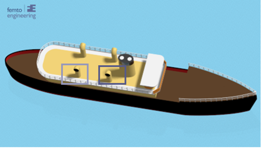
Figure 2: cabin inlets of interest
In Figure 3 the results of the simulation are shown for both the passive scalar method as well as the multicomponent gas method. In figure Figure 3 (top) the total amount of CO2 over time flowing in the cabin is shown. This table indicates that the total amount of CO2 entering the cabin greatly exceeds safe values within the first 20 seconds, but afterwards reduces significantly. Note that this table shows that added amount of CO2 compared to a baseline value of 0. Since the baseline amount of CO2 in the air is already around 400ppm, this value should be added to the table to correctly conclude if an unsafe working environment is created.
This table indicates that if the ship starts moving with a windspeed of 3.5m/s which comes under an angle of 30° , after which the wind speed reduces while the ship increases in speed to keep the angle of 30° this graph will give a good indication of the climate within the cabin. After a minute the total amount of CO2 in the cabin is still reducing, which means that once the ship reaches a constant velocity, the cabin climate will be sufficient for people to be there.
In Figure 3 (middle) and Figure 3 (bottom) the total amount of the other exhaust gas components for both simulation methods is shown. From these graphs it can be concluded that the passive scalar method under predicts the peak values of the exhaust gases entering the cabin. However, after a minute the values found by the passive scalar method are equal to the values found by the multicomponent gas method. Therefore, it can be concluded that if an equilibrium value is needed, that both methods work equally well. However, if peak values are very important, the multi-component gas method is better.
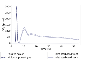
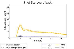
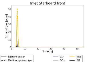
Figure 3: CO2 flowing into the cabin inlets (top), exhaust gas components flowing into the starboard back cabin inlet (middle), exhaust gas components flowing into the starboard front cabin inlet (bottom).
In Figure 4 the difference between the multicomponent gas and the passive scalar at the inlet height is shown. The difference in CO2 at these heights and this simulated time is very minor.

Figure 4: CO2 values at the cabin inlet height after a minute of simulated time